DBscan

Clustering Algorithm

Clusters are dense regions in the data space, separated by regions of the lower density of points. The DBSCAN algorithm is based on this intuitive notion of “clusters” and “noise”. The key idea is that for each point of a cluster, the neighborhood of a given radius has to contain at least a minimum number of points.

Parameters Required For DBSCAN Algorithm

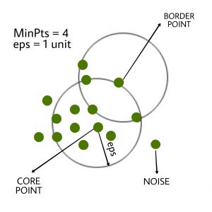
1. eps: It defines the neighborhood around a data point. One way to find the eps value is based on the k-distance graph.

   

   eps area
2. MinPts: Minimum number of neighbors (data points) within eps radius. As a general rule, the minimum MinPts can be derived from the number of dimensions D in the dataset as, MinPts >= D+1. The minimum value of MinPts must be chosen at least 3.

Data points

In this algorithm, we have 3 types of data points. Core Point: A point is a core point if it has more than MinPts points within eps. Border Point: A point which has fewer than MinPts within eps but it is in the neighborhood of a core point. Noise or outlier: A point which is not a core point or border point.

---

Example:

import numpy as np
import matplotlib.pyplot as plt
from sklearn.datasets import make_moons
from sklearn.cluster import DBSCAN

# Generate synthetic moon-shaped data
X, _ = make_moons(n_samples=1000, noise=0.1, random_state=42)

# Apply DBSCAN clustering
dbscan = DBSCAN(eps=0.2, min_samples=5)
y_pred = dbscan.fit_predict(X)

# Plot the clusters
plt.figure(figsize=(8, 6))
plt.scatter(X[:, 0], X[:, 1], c=y_pred, cmap='viridis', marker='o', edgecolors='k')
plt.title('DBSCAN Clustering')
plt.xlabel('Feature 1')
plt.ylabel('Feature 2')
plt.show()

---

Visualization

import matplotlib.pyplot as plt  #treba da se ispravi!!!

plt.scatter(X[:, 0], X[:, 1])
plt.show()